

SAMSON provides various visualization tools (visual models, visual presets, etc.) and rendering options (styles, special effects, etc.) to help you analyze molecular systems and create beautiful visualizations and animations.
You can try the following interactive tutorials in SAMSON (Help menu > Tutorials): "Visualization: visual models and colorization", "Visualization: rendering parameters".
See also: Selecting, Colorizing, Visual models, Visual presets, Rendering using Cycles, Presenting and animating
In this section, you will learn how to use SAMSON's visualization tools and rendering options.
Prerequisites:
- Please refer to the Selecting section to learn how to select nodes in SAMSON.
- Please refer to the Inspecting section to learn how to inspect nodes in SAMSON.
Applying visual presets
The fastest way to visualize a molecular system is by applying visual presets to it. Visual presets provide an efficient way to apply multiple visual representations and color schemes simultaneously to a complex molecular system based on selectors, all in just a few clicks. SAMSON provides a set of default visual presets and you can create and save your own visual presets, e.g., by modifying the existing ones. See the Visual presets section on how to apply and create visual presets.
To apply a visual preset click on Visualization menu > Visual model > Visual preset and, in the pop-up window, select a visual preset among the existing ones and click apply.
The visual preset is applied to the selected nodes or to the whole document if nothing is selected. The visual models created by the visual preset are stored in the document in a folder named based on the visual preset.
In the example below, the receptor is shown as ribbons, ligands and waters are represented as licorice, and ions are shown through a van der Waals representation in just a few clicks.
Please refer to Visual presets section for more information on how to apply visual presets and create your own visual presets.
Further in this section you will learn how to apply visual models, colorize, and change various rendering effects.
Applying illustrative style
If you would like to apply an illustrative visualization and rendering style inspired by the RCSB PDB Molecule of the Month style by David S. Goodsell (RCSB PDB-Rutgers and The Scripps Research Institute) follow these steps:
- to apply the illustrative visualization style, click Visualization menu > Visual model > Visual preset and, from the visual presets, select Illustrate... which would apply the van der Waals visual model for receptors and ligands with the color per chain ID (illustrative) and the van der Waals model for ions.

- to apply the illustrative rendering style, click Visualization menu > Presets > Illustrative which would set the rendering preferences to resemble the illustrative style.
To reset the view and the rendering style, remove the applied visual models in the Document view and in Visualization menu > Presets choose Default or High quality as shown in the Changing rendering presets subsection.
Changing rendering presets
SAMSON provides several predefined rendering presets between which you can easily switch in Visualization menu > Presets.
Rendering presets make it possible to quickly switch between different sets of special rendering effects like ambient occlusion, lighting, fog, shadows. You can also easily change these rendering effects in Visualization menu > Options or directly in Preferences as described in the Special effects section.
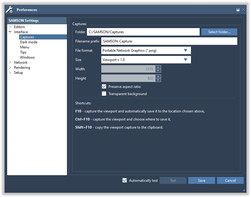
Capturing viewport
To save a picture, you can capture the viewport:
- Press F10 to take the viewport capture, the captured image is saved in the folder specified in capture preferences.
- Press Ctrl / Cmd⌘ + 10 to take the viewport capture and choose where to save it.
- Press Shift + 10 to copy the viewport capture to the clipboard.
You can modify the capture preferences in the Preferences > Interface > Captures panel (Interface menu > Preferences).
Hiding and showing nodes
You can hide from displaying in the viewport any group of structural nodes (atoms, chains, residues, molecules, etc.), folders, visual models, meshes, labels, and some other nodes. When you hide a parent node its descendants will be automatically hidden as well, e.g. if you hide a residue then atoms in this residue will be hidden, but you can make descendant nodes visible while their parent node is hidden.
You can hide a node just by unchecking the box of this node in the document view. For example, in the image below the chain B is hidden and won't be visible in the viewport. You can show a node by checking the box back.
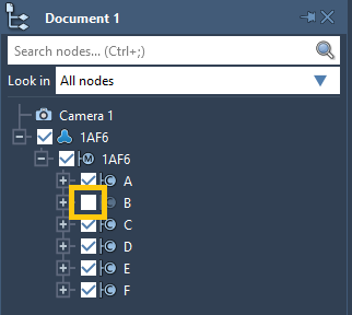
Note: If at least one descendant of a node is visible then the node's box in the document view will be shown as ticked to depict that some of its descendants are visible.
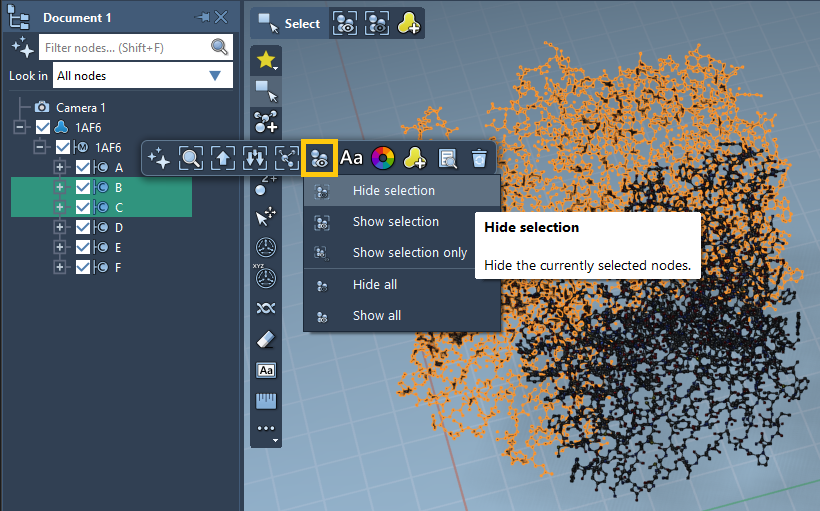
To change the visibility of nodes, select them in the document view or in the viewport, then in the context toolbar go to the ![]() Visibility section where you can change the visibility of the selection and of all nodes. For example, in the image below we are to hide the two selected chains.
Visibility section where you can change the visibility of the selection and of all nodes. For example, in the image below we are to hide the two selected chains.
Also, you can hide/show nodes using Python Scripting.
Transparency
For some nodes (structural models, folders, labels, and many visual models, meshes) you can modify their transparency by selecting them and changing this parameter in the Inspector.
Here is how, a semi-transparent structural model might look like along an opaque secondary structure visual representation:
Representation of atoms and bonds
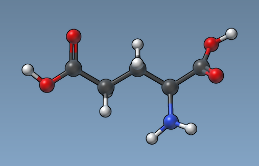
Atoms and bonds in structural models have a default visual representation, where atoms are represented as balls and bonds as sticks.
You can modify it in Preferences > Rendering > Structural models:
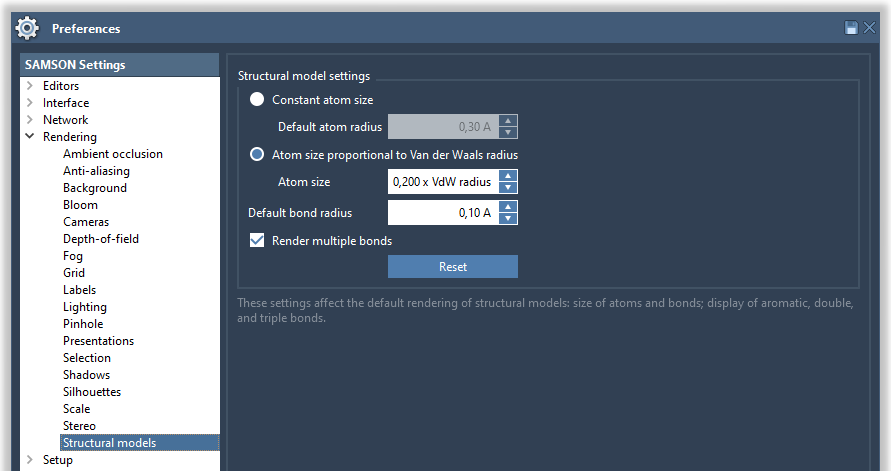
Try various options, constant atoms size or atom size proportional to van der Waals radius, and various parameters for atom and bond sizes to see how it affects the display of molecules. If the Automatically test box is checked, this immediately affects the rendering in the viewport.
For example, here is how a molecule looks like with the "Constant atom size" option and the default atom radius (0.3Å):
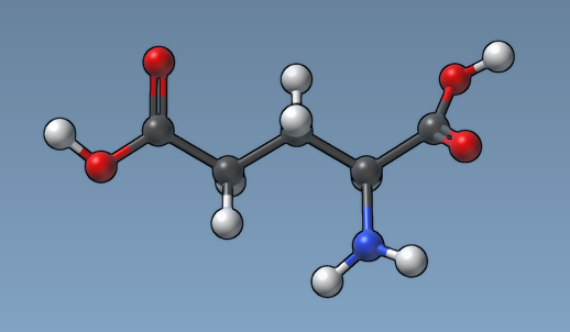
And here how the same molecule looks like with the "Atom size proportional to van der Waals radius" option.
Adding visual models
Visual models provide alternate visual representations of structural models, or even some arbitrary shapes, that may be displayed in the viewport.
Let's open a molecule, e.g. 1AF6 using Home menu > File > Fetch which will download it from RCSB PDB. We will apply a Ribbons (secondary structure) visual model to it.
Important: When a new visual model is added to the document, it is applied to the current selection, or, if nothing is selected, to the whole document. So, before adding a visual model make sure that a system to which you would like to apply it is selected and nothing else is selected, or nothing is selected if you would like to apply it to everything in the document.
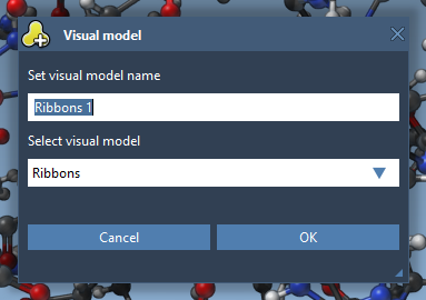
Visual models may be added from the Visualization menu (Visualization > Visual model) or via Ctrl / Cmd⌘ + Shift + V . A pop-up menu will appear asking you to choose a visual model type and provide a name for a visual model node that will be created. For example, let's choose the Ribbons (secondary structure) visual model.
As a result, a new visual model will be added in the document. You can also hide the structural model by unchecking its box in the document view.
Provided they handle them, visual models can be colorized with color schemes. This is the case for the Ribbons (secondary structure) visual model which we added before (when no color scheme is applied, a default color scheme based on the residue sequence numbers is used, as in the picture above). For more information see the Colorizing section.
As other node, you can colorize a visual model in several ways:
- Select the visual model and, in its context toolbar, set the material
 .
. - Select the visual model and apply a color scheme from Visualization menu > Material.
- Select the visual model and change/apply a color scheme in the Inspector.
In the example below, we apply different color schemes to the Ribbons visual model using the above-mentioned ways.
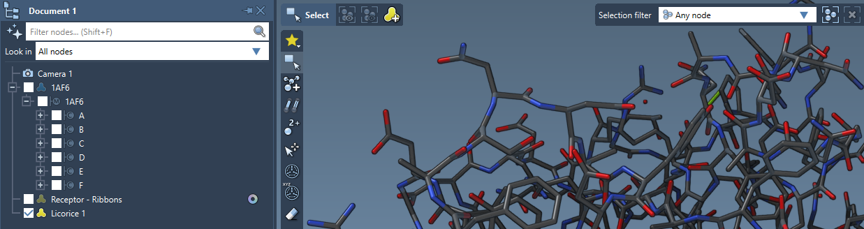
You can apply several visual models at once even to the same nodes. For example, try applying the Licorice visual model: select a molecule, click Ctrl / Cmd⌘ + Shift + V , and choose the Licorice visual model.
Colorizing
See the Colorizing section.
Special effects
See the Rendering effects section.
Examples
Dengue virus
Let's make the following image of the molecule with PDB code 3J27 (part of the Dengue virus):
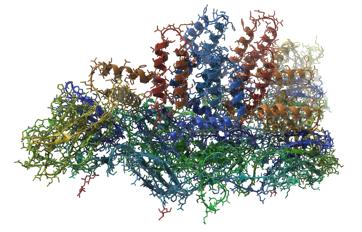
You can reproduce this image via the following steps:
- Add the Ribbons (secondary structure) visual model ( Ctrl / Cmd⌘ + Shift + V ).
- Add the Licorice visual model.
- Hide the structural model of the molecule.
- Orient the molecule in the viewport, you can for it use the Compass in the bottom-left corner of the viewport.
- Colorize the Licorice visual model by the residue index (select the Licorice visual model and in the context toolbar choose Material > Per attribute > Residue index).
- Ambient occlusion: enable object-space ambient occlusion with the default parameters.
- Anti-aliasing: enable with multisampling factor set to 2, enable FXAA.
- Background: white.
- Fog: enable with the far distance parameter set to 100Å.
- Lightning: default parameters for the first and second lights; set ambient light to 0.
- Shadows: enable with the default parameters.
- Silhouettes: disable.
The nucleosome core particle
Let's make the following image of the molecule with PDB code 1EQZ (the nucleosome core particle):
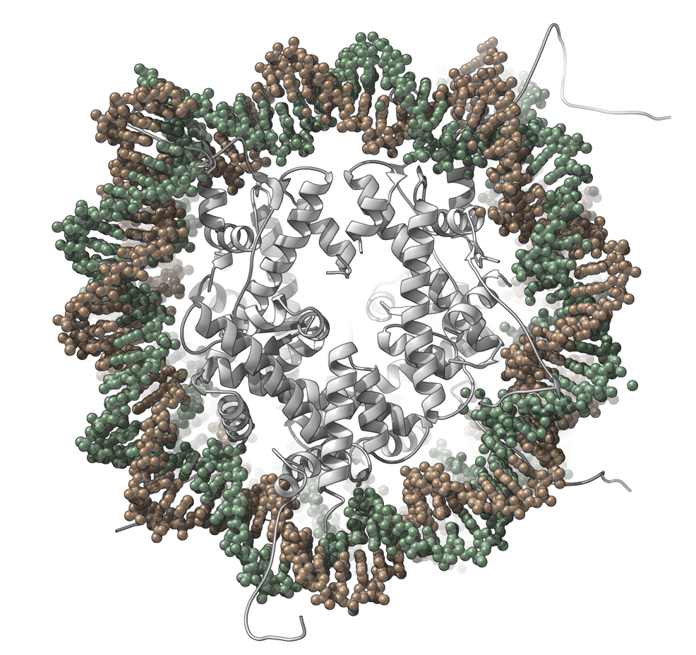
You can reproduce this image via the following steps:
- Orient the molecule in the viewport, you can for it use the Compass in the bottom-left corner of the viewport.
- In the document view, expand the molecule to see chains. Select chains from A to H and apply the Ribbons (secondary structure) visual model ( Ctrl / Cmd⌘ + Shift + V ), and then hide the selection.
- Select the Ribbons (secondary structure) visual model and colorize it with a constant color (white).
- Open Preferences, modify the structural models representation (Rendering > Structural models): set the atom radius to 1Å.
- Select the chain I and colorize it with a constant color. Colorize the chain J with a constant color.
- Ambient occlusion: disable.
- Anti-aliasing: enable with multisampling factor set to 2, enable FXAA.
- Background: white.
- Fog: enable with the default parameters.
- Lightning: default parameters.
- Shadows: enable with the default parameters.
- Silhouettes: enable and set the silhouette opacity to 60%.
Pilus machine
Let's reproduce an image of the molecule with PDB code 3JC8 (the type IVa pilus machine in a piliated state).
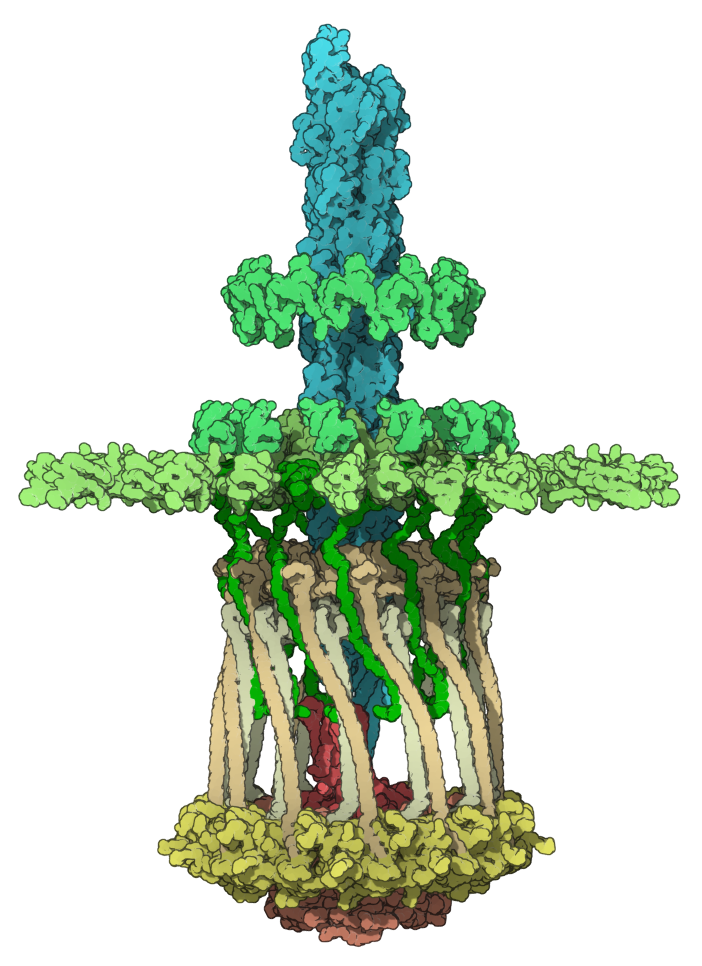
Here we colorized 3JC8 by groups of chains. Please, download 3JC8.sam file in which for simplicity we combined chains in groups.
You can reproduce this image via the following steps:
- Orient the molecule in the viewport, you can for it use the Compass in the bottom-left corner of the viewport.
- Open Preferences, modify the structural models representation (Rendering > Structural models): set the atom radius to 3Å.
- Colorize each group of chains: double-click on the group and colorize it with a constant color.
- Ambient occlusion: enable object-space ambient occlusion with the default parameters.
- Anti-aliasing: enable with multisampling factor set to 2, enable FXAA.
- Background: white.
- Fog: disable.
- Lightning: the light intensity for first and second lights is set to zero; the ambient light is set to 1 and the Fresnel intensity is set to 0.
- Shadows: enable with the default parameters.
- Silhouettes: enable, set the silhouette opacity to 60%, the silhouette thickness to 1, and the distance threshold to 2Å.
DNA polymerase with DNA
Let's make the following image of the molecule with PDB code 4QWE (DNA polymerase in complex with DNA).
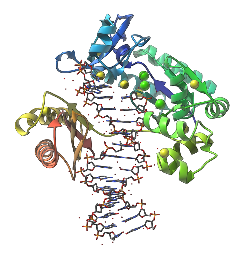
You can reproduce this image via the following steps:
- In the document view, expand the molecule to see chains. Select the chain A and apply the Ribbons (secondary structure) visual model ( Ctrl / Cmd⌘ + Shift + V ), and then hide the selected chain.
- Find all Sulfur and Calcium atoms. Open the Find window (Select menu > Find or Ctrl / Cmd⌘ + F ). Input
atom.symbol S or atom.symbol Ca(short version:a.s S or a.s Ca) and click Enter . Now you should see 11 nodes selected, press Ctrl / Cmd⌘ + Shift + V and add Van der Waals visual model. Select in the document view the newly created Van der Waals visual model and in the Inspector (click Ctrl / Cmd⌘ + I if you do not see the Inspector) set the scale to 0.75. - In the document view, select the chains C and D and apply to them the Licorice visual model.
- Ambient occlusion: disable.
- Anti-aliasing: enable with multisampling factor set to 2, enable FXAA.
- Background: white.
- Fog: enable with the far distance set to 50Å.
- Lightning: default parameters.
- Shadows: enable with the default parameters.
- Silhouettes: enable and set the silhouette opacity to 50%.
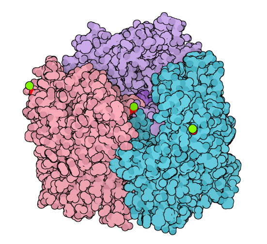
The human erythrocyte catalase
Let's make the following image of the molecule with PDB code 1DGF (the human erythrocyte catalase).
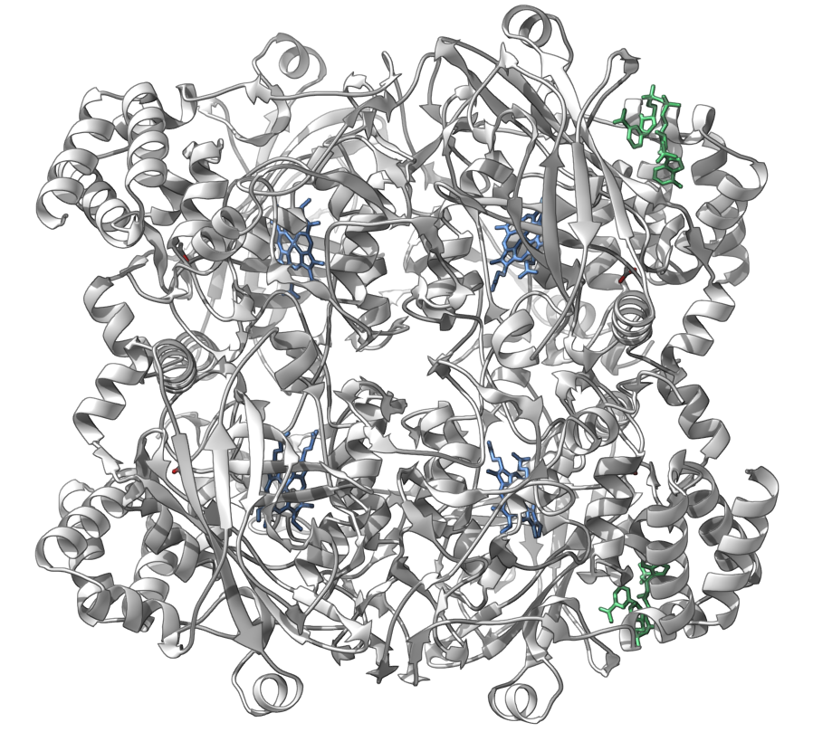
You can reproduce this image via the following steps:
- Add the Ribbons (secondary structure) visual model ( Ctrl / Cmd⌘ + Shift + V ).
- Let's now hide all residues and water atoms, leaving shown only ACT, HEM, and NDP structural groups. Open the Find window (Select menu > Find or Ctrl / Cmd⌘ + F ). First we will hide all non structural groups: input
n.t structuralGroup(short version:n.t sg) and click Enter , then right-click on any selected node, and choose Invert selection in the context menu, then using the context toolbar for the selection choose Visibility > Hide selection. Let's now hide all water atoms: open the Find window, inputa.waterand click Enter , then in the context toolbar choose Visibility > Hide selection. - Open Preferences, modify the structural models representation (Rendering > Structural models): set atom and bond radius to 0.3Å.
- In the document view, select the Ribbons (secondary structure) visual model and colorize it with a constant color (white).
- Let's colorize HEM and NDP structural groups. In the document view, enter HEM in the Filter nodes... and click Enter . Colorize it with constant color. Do the same for the NDP structural groups.
- Ambient occlusion: disable.
- Anti-aliasing: enable with multisampling factor set to 2, enable FXAA.
- Background: white.
- Fog: enable with the far distance set to 50Å.
- Lightning: default parameters.
- Shadows: enable with the default parameters.
- Silhouettes: enable and set the silhouette opacity to 50%.
- Orient the molecule in the viewport.
See also: Color schemes See also: Visual models See also: Visual presets See also: Presenting and animating