


In this post, we will show how to use the Ligand Path Finder app for finding possible ligand unbinding pathways from a protein.
Content
- Requirements
- Tutorial
- Loading the input model
- Launching the Ligand Path Finder app
- Setting up the interaction model and the state updater for energy evaluation
- Setting up the system
- Defining the sampling box
- Defining the parameters
- Running, pausing, or stopping the planner
- Results
- Next steps
Requirements
- SAMSON version 2020 R1 or higher
- Ligand Path Finder app
- GROMACS force field interaction model
- FIRE state updater
Before starting the tutorial, please, download the LigandPathFinder sample archive which contains necessary files for this tutorial. After extracting it, you will have a structural model (1pv7_ligand_complex.sam) and the topology files for energy evaluation with Gromacs (1pv7_ligand.itp, 1pv7_ligand_complex_topol.top, 1pv7_posre.itp).
Tutorial
In this tutorial, we will apply the ART-RRT method for finding ligand unbinding pathways from a protein. The ART-RRT method is a combination of the T-RRT method and the ARAP modeling method. The T-RRT method is used for finding possible pathways and the ARAP modeling method is for generating possible ligand motions. Moreover, a constrained minimization is used for adapting the motion of the protein with the ligand.
Loading the input model
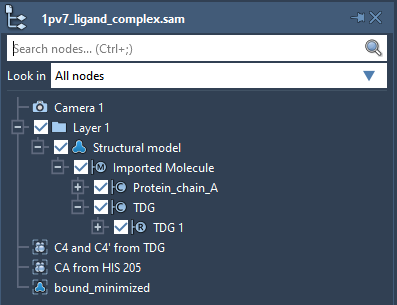
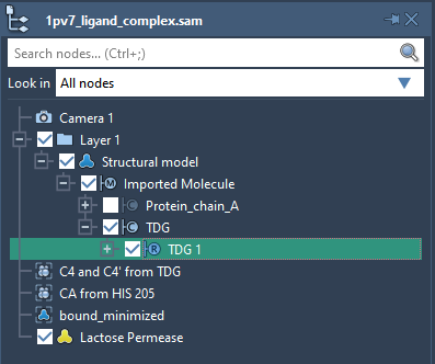
Launch SAMSON. Load 1pv7_ligand_complex.sam. It will open a structural model of Lactose permease with its ligand Thiodigalactosid. In the Document View (if you do not see it, enable it in the Window menu, or press Ctrl+1), you can see the protein under the name Protein_chain_A and the ligand under the name TDG as shown in the picture below. You also can see one conformation named bound_minimized which is the minimized conformation of the protein-ligand complex.
Visualizing the secondary structure of the protein
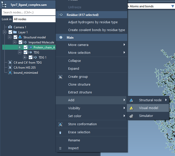
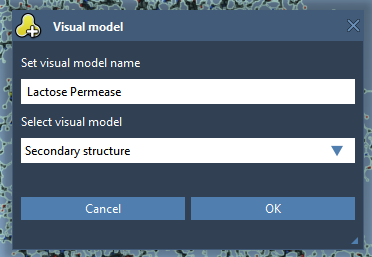
Let’s create a secondary structure for the protein. In the Document View, right-click on the Protein_chain_A and choose Add > Visual Model. In the Add visual model window, select visual model to be Secondary structure as shown in the following figure.
Let’s now hide the default ball-and-stick representation of the protein for better visibility by unchecking the box next to the Protein_chain_A in the Document View.
Launching the Ligand Path Finder app
Open the Ligand Path Finder app by clicking on its icon ![]() (you can also find it in the App > Biology menu).
(you can also find it in the App > Biology menu).
In the app’s window, you can see two tabs: the Settings tab is for configuring the search and the Results tab is for visualizing results.
Setting up interaction and state updater models for energy evaluation
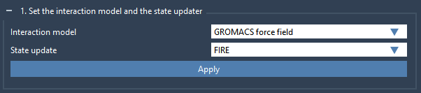
First, in the Settings tab, we need to specify an interaction model and a state updater which will be used in the computations. For the Interaction model select GROMACS force field in the drop-down list, and for the State updater select FIRE. If you do not see either GROMACS force field or FIRE state updater, please check the requirements section and make sure you installed all necessary SAMSON Elements.
Then click Apply button (see the figure below). This will apply the interaction model and state updater on all the atoms in the document.
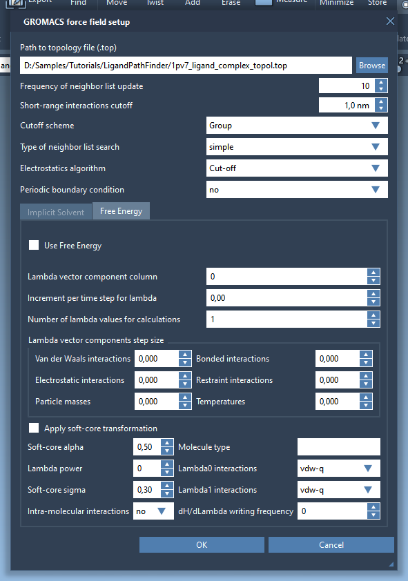
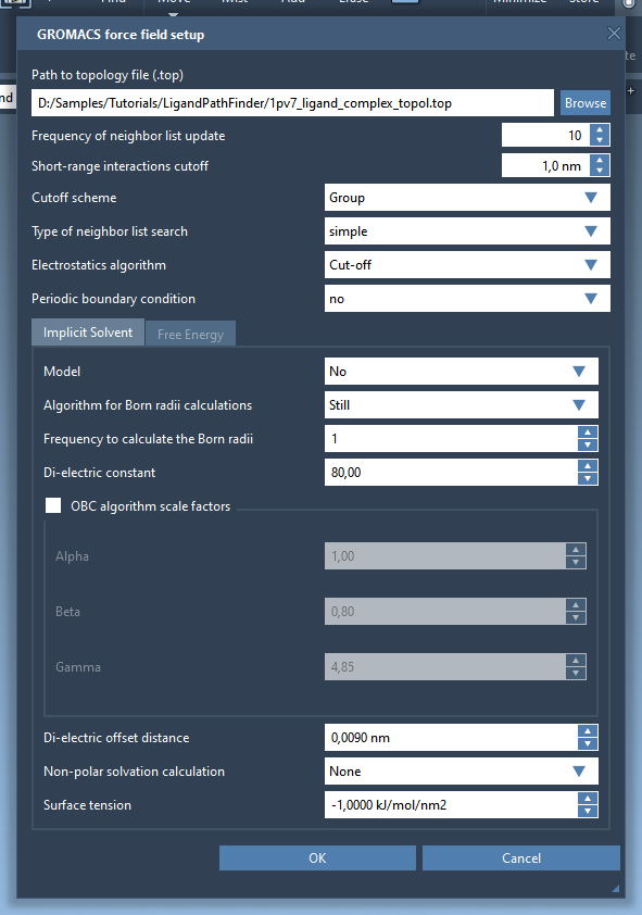
A window will pop up asking if you want to apply a new model, click Yes. The GROMACS force field setup will then ask for the topology file for the protein-ligand model. Click Browse and choose to open the file 1pv7_ligand_complex_topol.top provided with the structural model file. Keep the rest of the information in the window intact (see the figure below) then click OK.
Two windows should appear: the GROMACS force field properties window showing the potential energy of the current state of the system and the FIRE Properties window showing the state updater parameters. Set the parameters for FIRE as in the picture below (the step size to 1 fs, the number of steps to 1).

Setting up the system
Let’s now set up the system. Expand the Set up of the system box.

Defining the bound state
Let’s choose the starting conformation. Select the bound_minimized conformation in the Document View and then, in the App, click Set as starting conformation. The chosen conformation will be considered as the starting state for the search tree.
![]()
Defining the ligand and active and fixed ARAP atoms
Defining the ligand atoms
Now we need to define the ligand. Select TDG in the Document view, this will select all the ligand atoms (see User guide: Selecting).
Then, in the App, click the Set button to set the ligand atoms.
![]()
The rest of the atoms will be considered as protein atoms.
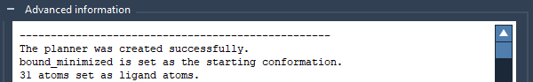
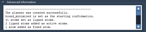
In the Advanced information box, a new line should appear: “31 atoms set as ligand atoms”.
Defining the active ARAP atoms
Now we need to specify which ligand atoms will be considered by the ARAP method as active atoms used for controlling the ligand motion. The motions of the rest of the ligand atoms (also called passive ARAP atoms) will follow these two active atoms. Let’s choose two Carbon atoms from the TDG ligand: C4 and C4’. For simplicity, the document contains a group named C4 and C4′ from TDG that refers to these atoms. In the Document view, double-click on this C4 and C4′ from TDG group. This will select nodes in the group, i.e. the C4 and C4’ atoms.
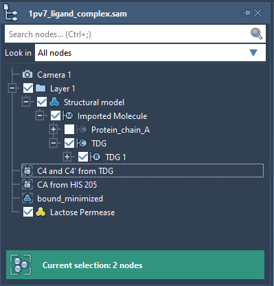
Then, in the App, click the Add button to set the active ARAP atoms.
![]()
Defining the fixed ARAP atoms
Finally, we need to specify which protein atoms will be considered by the ARAP method as having a fixed position. This is to ensure that the protein will not drift along with the ligand (note that this choice may influence the resulting unbindings pathways, so in general you should choose atoms from parts of the protein that are expected to be rather static).
Let’s choose the CA atom in the Backbone of HIS 205 residue of the protein as the fixed ARAP atom. For simplicity, the Document has a group named CA from HIS 205 that refers to this atom. In the Document view, double-click on this group to select the corresponding atom.
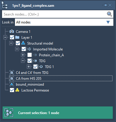
Then, in the App, click the Add button to set the fixed ARAP atom.
![]()
In the Advanced information box, you should see the number of added active and fixed ARAP atoms.
You can see which atoms were chosen as ligand, active or fixed ARAP atoms by clicking the corresponding Select and Unselect buttons. If you are not satisfied with the starting conformation selection, ligand atom selection, or atom type assignment, you can reset your choices by clicking the corresponding Reset (![]() ) button.
) button.
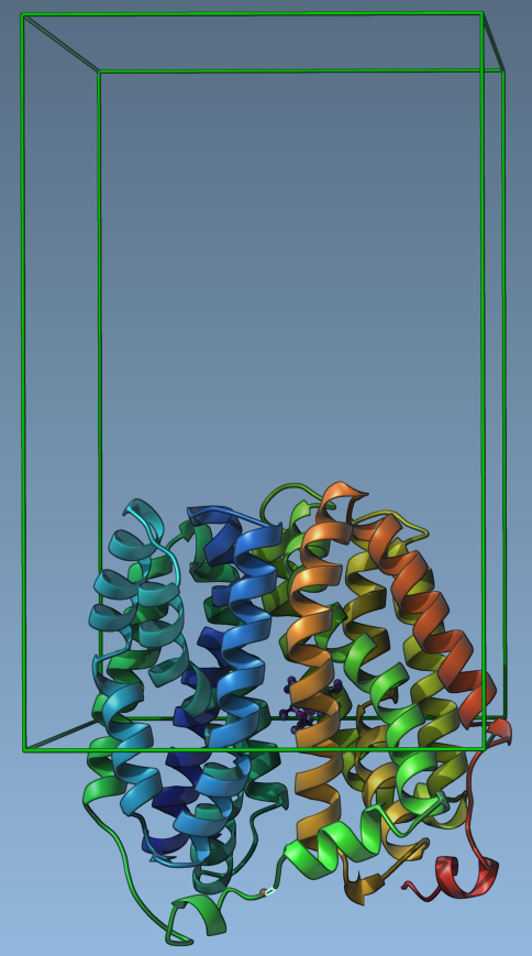
During the setup of the system, a new visual model should appear for showing the sampling box and atom types (blue for passive ARAP atoms, green for active ARAP atoms, and red for fixed atoms).
Defining the sampling box
Let’s now define the sampling box for the active ARAP atoms. Expand the Set the sampling box for the active ARAP atoms box.
The sampling box defines the sampling region for the chosen active ARAP atoms. The size and position of the box biases the ligand motion and therefore the resulting unbindings pathways. The App suggests the sampling box size which encloses the ligand and protein atoms. Let’s set the sampling box dimension as follows (this box dimension biases the ligand motion towards the periplasmic side of the protein):
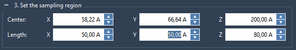
A green box visualizes the sampling box.
Defining the parameters
Let’s now define the parameters. Expand the Set parameters box and set them as in the following figure:
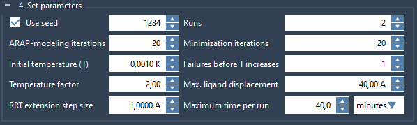
- Use seed is checked and the value is 1234: we use the specified seed number for the planner and after each run the seed value is incremented by 1. If the box is unchecked, a random seed is used.
- Runs = 2: we run the method 2 times to extract a maximum of 2 paths.
- ARAP-modeling iterations = 20: the number of iterations for the ARAP modeling method.
- Minimization iterations = 20: apply 20 steps of constrained minimization with FIRE each time a new state is sampled to minimize it.
- Initial temperature (T) = 0.001 K, Temperature factor = 2, Failures before increase of T = 1 : parameters for T-RRT.
- Max. ligand displacement = 40 A: each run is stopped as soon as the center of the ligand is displaced by 40 angstrom from its original position.
- RRT extension step size = 1 A: the size of the extension step is 1 angstrom. This affects how fast the conformation space is sampled.
- Maximum time per run: each run is stopped as soon as the elapsed time reaches this value.
Running, Pausing, or Stopping the planner
Once you set up the system, the sampling box, and specified the parameters, you can launch the search for ligand unbinding pathways.
Click the Run button to start the planner. The search process can be paused by clicking the Pause button and resumed after that by clicking on the Resume button (these buttons are located at the same place as the Run button while the planner is running). To stop the process, click the Stop button.
During the search, in the Advanced information box under the Planning information, you can observe the elapsed time for the current run (Current running time), the elapsed time for all of the runs (Total running time), the number of nodes of the tree in the current run (Nodes), the run number (Run), and the number of paths found (Paths found).

Results
As soon as a path is found, it is added to the list in the Results tab. For example, the following figure shows two paths found.
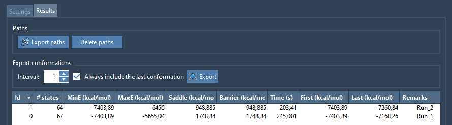
Each path contains the following fields
- id: path id
- # states: Number of conformations in the path.
- MinE (kcal/mol): Minimum energy of the path conformations.
- MaxE (kcal/mol): Maximum energy of the path conformations.
- Saddle (kcal/mol): Difference between MaxE and MinE.
- Barrier (kcal/mol): Difference between MaxE and First.
- Time (s): Time elapsed for searching this path.
- First (kcal/mol): Energy of the first conformation in the path.
- Last (kcal/mol): Energy of the last conformation in the path.
- Remarks: Comments on the path (editable).
- Color: Color of the energy curve for this path.
Viewing conformation energies along the path
To view the energy curve of the path, select a path by clicking on it in the path table. To plot several energy curves, select several paths (Ctrl / Cmd + left-click for multi-selection). After selecting a path, you can move the slider to see a particular conformation in the path as shown in the picture below. The corresponding conformation is reflected in the structural model in SAMSON and its corresponding energy is shown in the GROMACS force field window.
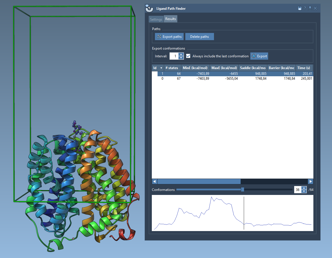
Exporting the results: paths, conformations, path table content
You can copy the content of the path table to the clipboard by selecting the paths for which you want to export data and pressing Ctrl / Cmd + C or right-clicking and choosing Copy table content. You can also copy path energy values along the selected paths via right-clicking and choosing Copy path energy.

To export paths from the path table into the document, select the paths you are interested in and press the Export paths button.
You can delete paths by selecting them in the path table and clicking the Delete paths button.
To export conformations along the path into SAMSON, select the paths from the path table, choose the export interval and click the Export button.
Next steps
Creating pathlines
Check the Pathlines tutorial to learn about how to create pathlines, for example to visualize the movement of the center of mass of a ligand.
Improving paths with P-NEB
The resulting paths can be significantly improved with the help of the parallel Nudged Elastic Band (NEB) method implemented in the P-NEB app. Please check out the P-NEB tutorial for more information.
Exporting atoms trajectories along paths
The resulting paths can be saved in the .sam and .samx formats. If you want to export only trajectories of some atoms along the path, you can use the Export Along Paths app. Please refer to the tutorial on how to use the Export Along Paths app for more information.
If you have any questions or feedback, please use the SAMSON forum.