

In this section, we will show how to use SAMSON's visualization tools and rendering options.
See also: Color schemes, Visual models, Visual presets, Presenting and animating
Hiding and showing nodes
In SAMSON you can hide from displaying in the viewport any group of atoms, chains, residues, molecules, and whole layers. When you hide a parent node its children nodes will be hidden as well, e.g. if you hide a residue then atoms in this residue will be hidden.
You can hide nodes from displaying in the viewport by selecting these nodes either in the viewport itself or in the document view. Also, you can hide/show nodes using Python Scripting.
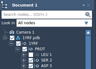
Let's open a molecule, e.g. 1YRF provided in the Samples folder or using the PDB Downloader.
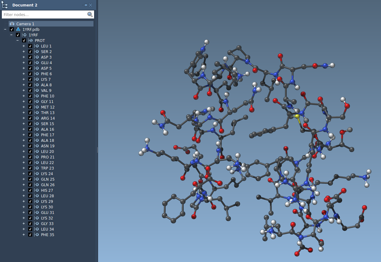
You can hide a node just by unchecking the box of this node in the document view. In the image below we hide the LEU 1 residue. You can show this node by checking the box.
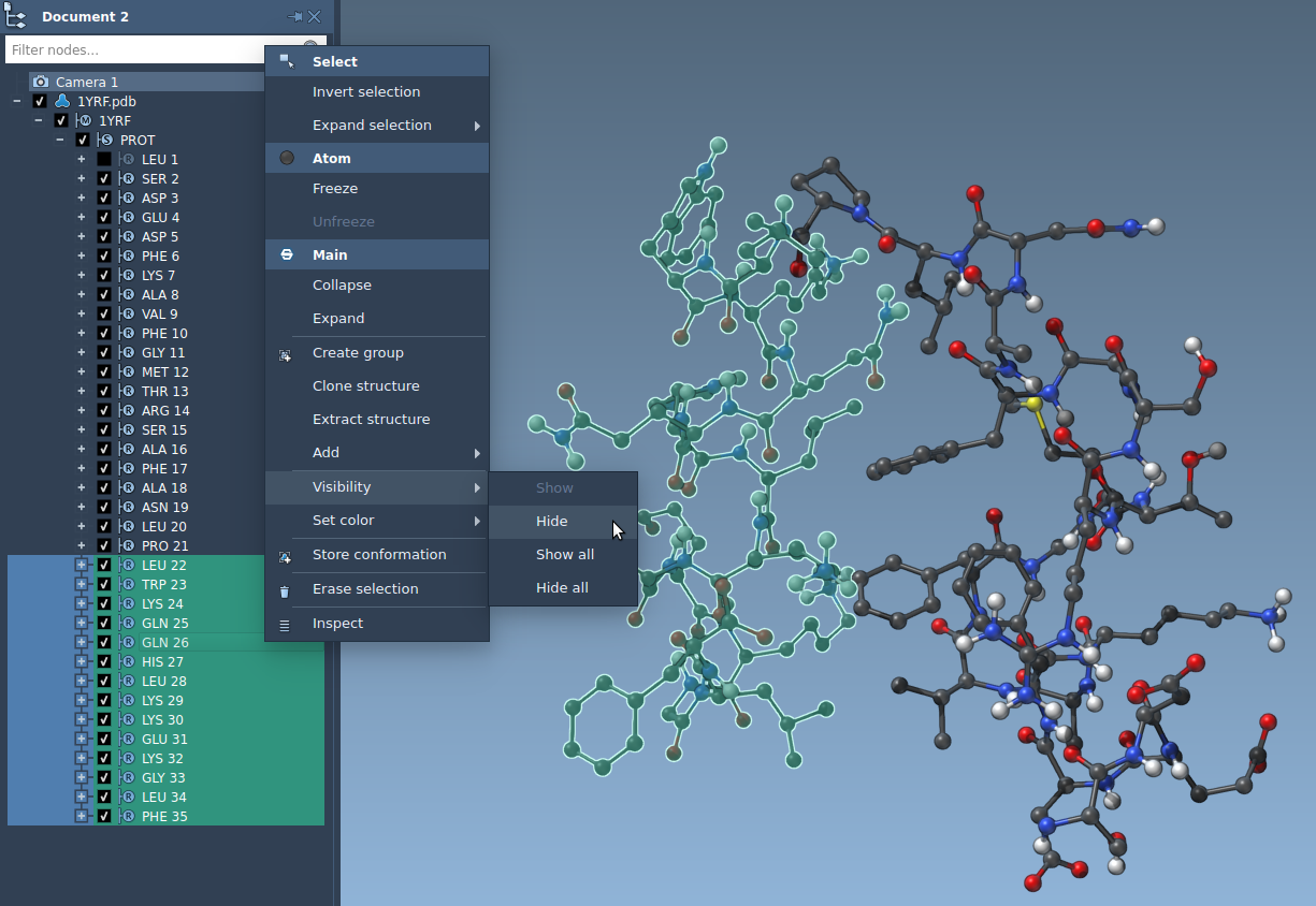
To hide or show a set of nodes, select them in the document view or in the viewport, then right-click and in the context menu go to the Visibility section where you can change the visibility of the selection and of all nodes. In the image below we hide a a set of residues.
Capturing viewport
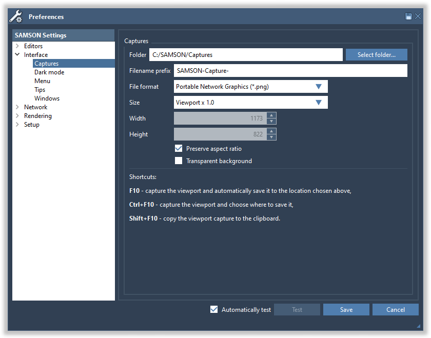
To save a picture you can capture the SAMSON's viewport by pressing F10. You can modify the capture preferences in the Preference panel (Interface menu > Preferences...), in the Interface / Captures section (see Captures preferences for more information).
You can also copy the viewport capture to the clipboard by pressing Shift+ 10.
Representation of atoms and bonds
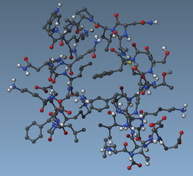
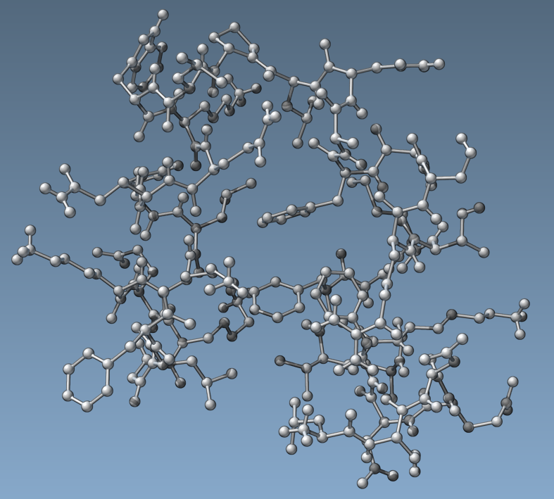
In SAMSON, molecules (structural models) have a default visual representation, where atoms are represented as balls and bonds as sticks.
Let's open a molecule, e.g. 1YRF provided in the Samples folder.
In the Preferences panel, go to the Rendering / Structural models section:
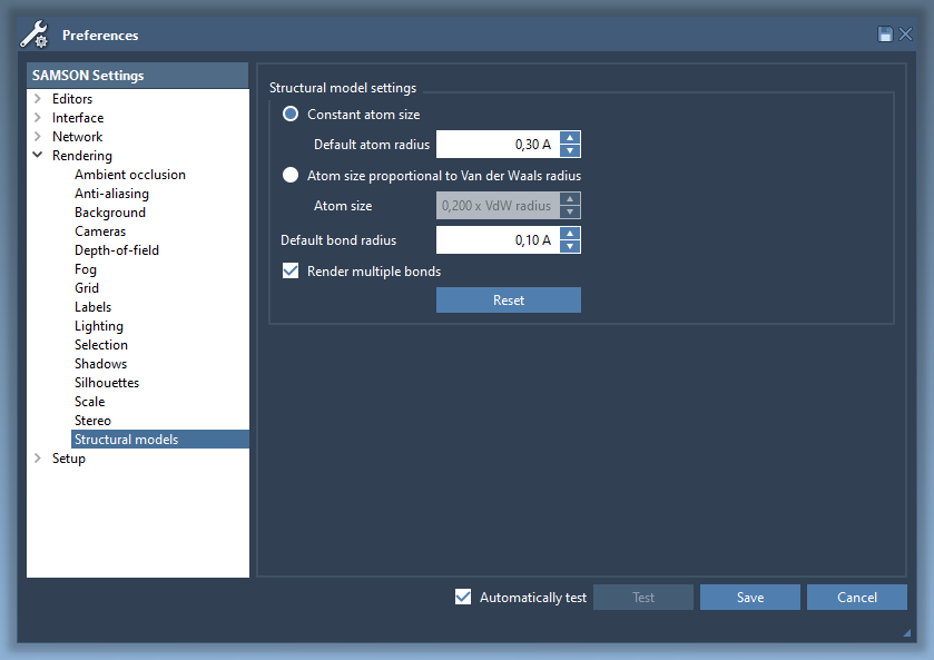
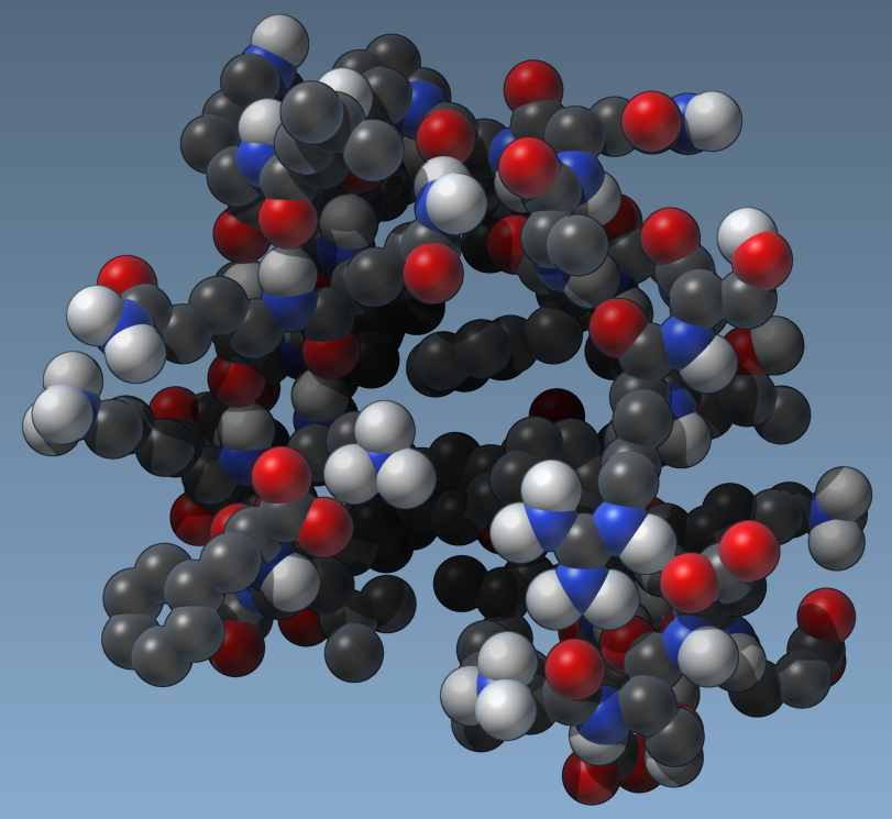
Change the default atom radius and bond radius. If the Automatically test check box is checked, this immediately affects the default rendering of the structural model. For example, let's set the atom radius to 1A:
Background color
The background color of the viewport may be changed in the Rendering / Background section of the Preferences panel:
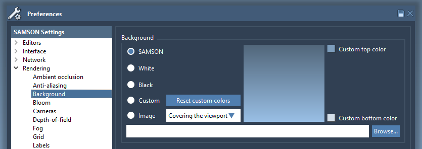
Four options are available:
- SAMSON: the default SAMSON background
- Black: an entirely black background
- White: an entirely white background
- Custom: a gradient from a user-defined top color to a user-defined bottom color
Let's try to set a custom gradient background by choosing Custom and modifying the Custom top color and the Custom bottom color.
You can switch betwenn different backgrounds easily in the Visualization menu and in the bottom of the Viewport.
You can always return to the default SAMSON background color.
Lightning
In SAMSON, lighting can be modified in the Rendering / Lightning section of the Preferences panel:
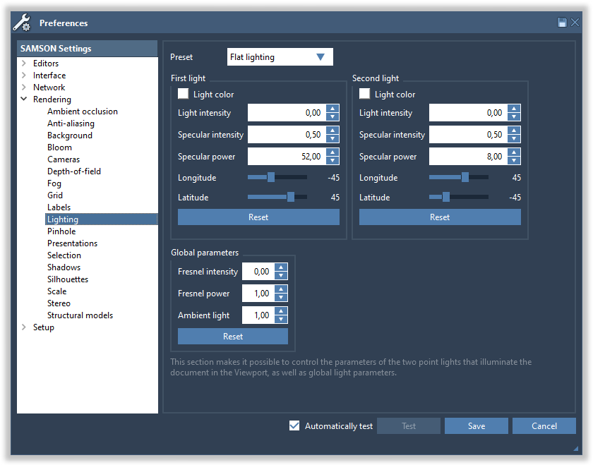
This section makes it possible to control the parameters of the two point lights that illuminate the document, as well as global parameters. Each light has the following parameters:
- Light color: click the square to change the color of the light
- Light intensity (between 0 and 1): the intensity of the light
- Specular intensity (between 0 and 1): the intensity of the light reflection on surfaces. High values make surfaces look like plastic, while low values make surfaces look matte.
- Specular power (between 0 and 1000): the decay of specular reflection. High values produce sharper specular reflections.
- Longitude and latitude control the position of the light.
The first light is typically the main light, which is thus typically brighter than the second light (a “back light”).
Finally, three more parameters are global:
- Fresnel intensity (between 0 and 1): the amount of background light reflected at grazing angles
- Fresnel power (between 0 and 100): how fast the Fresnel effect decays
- Ambient light: the amount of light that reaches objects, even when the intensity of both lights is set to 0.
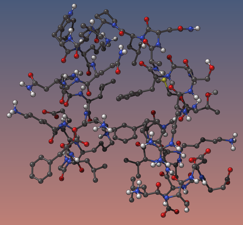
Try changing all parameters and see the impact on rendering (switch on the Automatically test check box in the bottom).
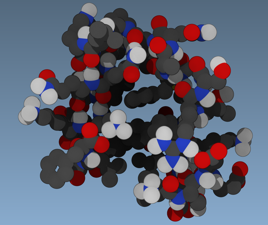
Let's modify the lights and global parameters to produce the following “flat” rendering. For that we set the light intensity for both first and second light to zero, the ambient light to 0.8, and the Fresnel power to zero.
Color schemes
In SAMSON, you can colorize structural nodes with a color scheme to modify the colors of atoms and bonds. Three types of color schemes are available:
- Constant: the same color is uniformly applied
- CPK: the classic Corey-Pauling-Koltun color scheme
- Per attribute: the color is determined based on an atom attribute (e.g. temperature factor, residue, etc.)
When a color scheme is applied to a node, all the node’s descendants are affected. You can apply different color schemes to different nodes.
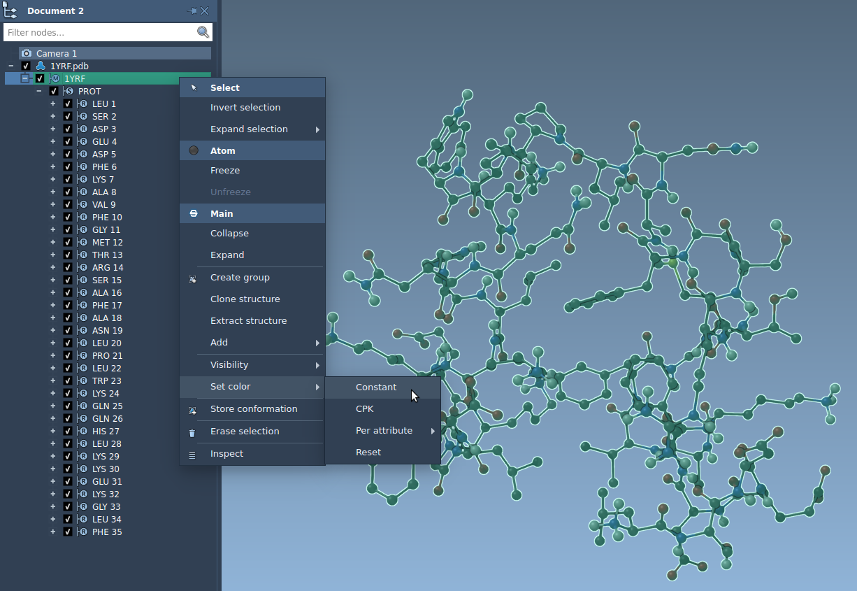
Let's open a molecule, e.g. 1YRF provided in the Samples folder. Select 1YRF in the document view, and first apply a constant color scheme: right-click and the Set color / Constant....
A dialog will appear in which you can choose the color.
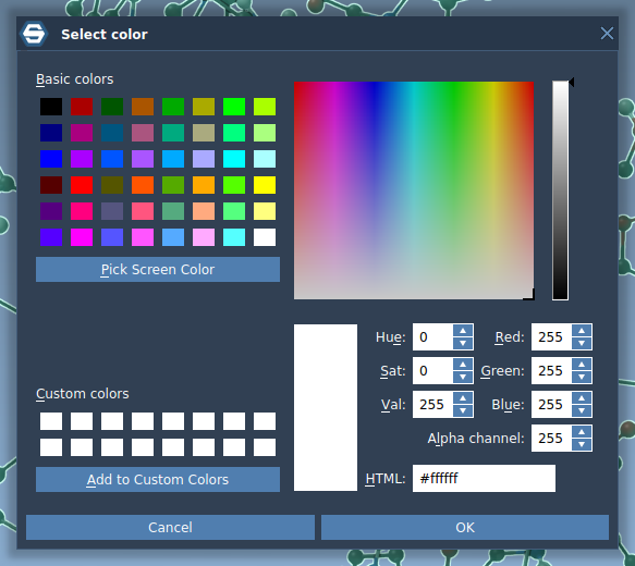
As a result, all the chosen nodes will be colorized with the same color.
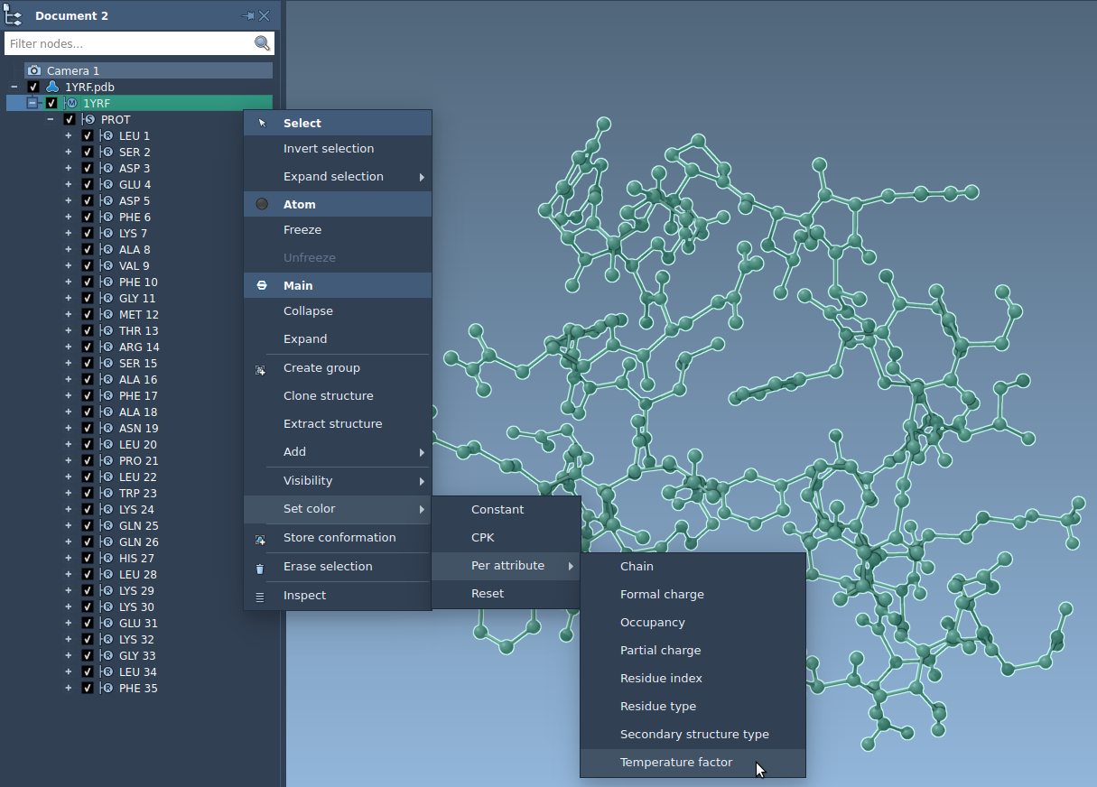
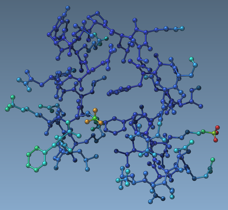
Let's now colorize according to the temperature factor. Select 1YRF in the document view, and in the context menu select Set color / Per attribute / Temperature factor.
As a result, all atoms will be colorized according to their temperature factor.
To reset the color scheme, select the node and in the context menu select Set color / Reset to go back to the default color scheme.
Adding visual models
In SAMSON, Visual models provide alternate visual representations of structural models, or even arbitrary shapes, that may be displayed in the viewport.
Important: when a new visual model is added to the document, it is applied to the current selection. If nothing is selected, it is applied to the whole document.
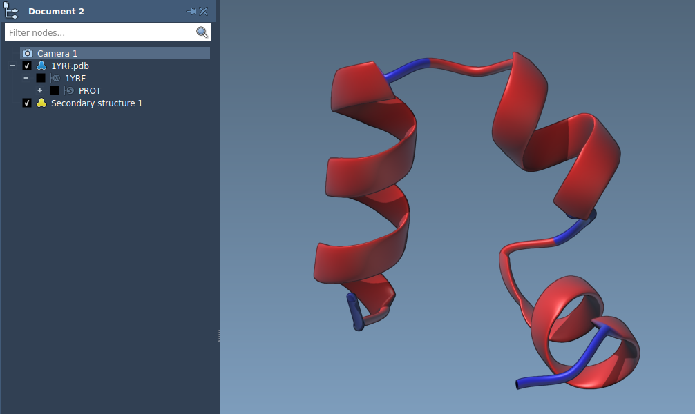
Let's open a molecule, e.g. 1YRF provided in the Samples folder, and apply a visual model to it. Deselect all or select 1YRF, and add a Ribbons (Secondary structure) visual model to the document. Then hide the structural model:
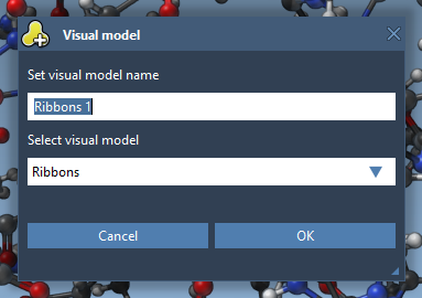
Visual models may be added from the Visualization menu (Visualization > Visual model) or via Ctrl/ Cmd⌘ + Shift + V. A pop-up menu appears to choose the name of the visual model and its type. Choose the Ribbons (secondary structure) visual model.
As a result, a new visual model will be added in the document. You can also hide the structural model by unchecking the box.
Provided they handle them, visual models can be colorized with color schemes. This is the case for the Ribbons (secondary structure) visual model (when no color scheme is applied, a defaul rainbow color scale based on the residue sequence numbers is used, as in the picture above).
Select the visual model, and colorize it by the secondary structure type. You should obtain the following image:
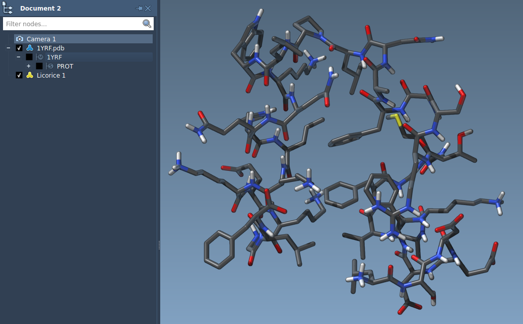
You can apply several visual models at once. Try applying the Licorice visual model: select a molecule, click Ctrl/ Cmd⌘ + Shift + V, and select the Licorice visual model.
Applying visual presets
Visual presets provide an efficient way to apply multiple visual representations and color schemes simultaneously to a complex molecular system, all in just a few clicks.
In the example below, the receptor is shown as ribbons, ligands and waters are represented as licorice, and ions are shown through a van der Waals representation in just a few clicks.
Please refer to Visual presets section for more information on how to apply visual presets and create your own visual presets.
Special effects
Several rendering effects may be applied from the Preferences panel.
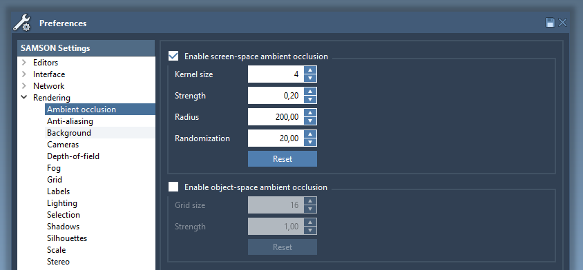
Ambient occlusion
Ambient occlusion improves the perception of depth in molecules, by simulating the fact that deeper regions are less accessible to light, and are thus darker.
Two types of ambient occlusion are handled in SAMSON:
- Screen-space ambient occlusion efficiently provides an approximate simulation, but is sensitive to the distance to the camera.
- Object-space ambient occlusion is more realistic, but slower. Even screen-space ambient occlusion is very useful to improve depth perception however.
The ambient occlusion settings may be changed in the Rendering / Ambient occlusion section of the Preferences panel:
The screen-space ambient occlusion can be switched on/off in one click in the Visualization menu.
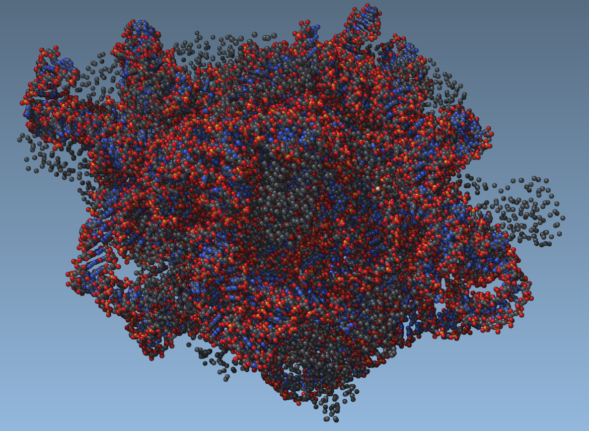
Here is 1FFK without ambient occlusion:
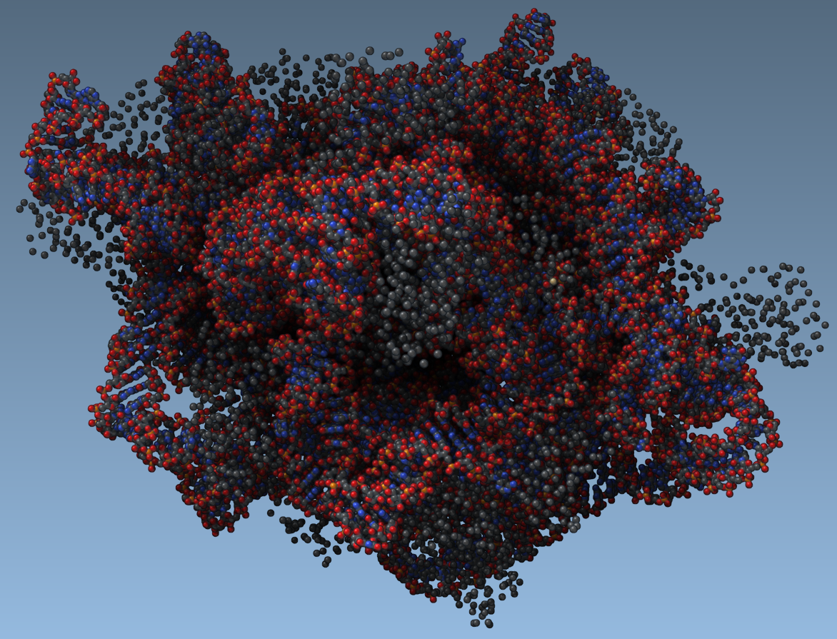
And here is 1FFK with enabled screen-space ambient occlusion:
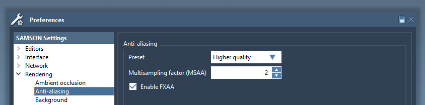
Anti-aliasing
Anti-aliasing removes jagged edges from images, and may significantly improve rendering. The anti-aliasing settings may be changed in the Rendering / Ambient occlusion section of the Preferences panel. Fast Approximate Anti-Aliasing (FXAA) is typically very efficient, and can be activated on most recent graphics cards.
Note: Anti-aliasing requires more rendering from your GPU and therefore may slow-down the visualization for big systems.
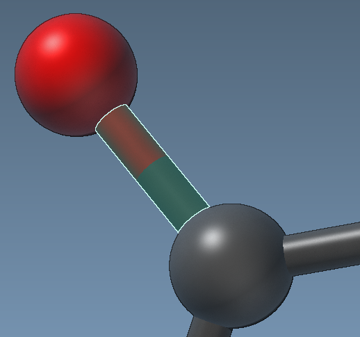
Without anti-aliasing (choose Best speed from the list: multisampling factor set to 1, no FXAA), edges are very visible:
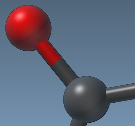
With FXAA and multisampling set to 2 (choose Higher quality from the list), edges are much smoother, and pixel boundaries are much less visible:
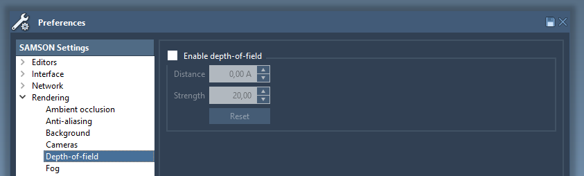
Depth-of-field rendering
This effect simulates the depth-of-field effect produced by actual cameras (e.g. blurred distant objects). If enabled, when you zoom in the molecule its distant parts will be blurred. The depth-of-field settings may be changed in the Rendering / Depth-of-field section of the Preferences panel:
Turn the depth-of-field on, set the strength to 80 and zoom on a molecule.
The depth-of-field can be switched on/off in one click in the Visualization menu.
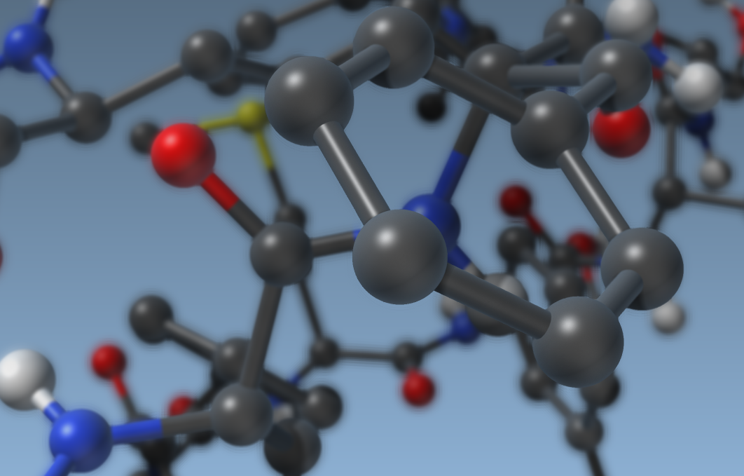
Fog
Basically, fog makes distant objects less visible. Fog attenuates distant parts by blending them progressively with the background. Turn it on to make it easier to focus on the foreground.
The near and far distances are based on the camera location and determine where the fog is enabled. Before the "near distance" there is no fog, after the "far distance" every node is invisible. The "strenght" parameter influences the speed at which the fog is appearing.
The fog settings may be changed in the Rendering / Fog section of the Preferences panel:
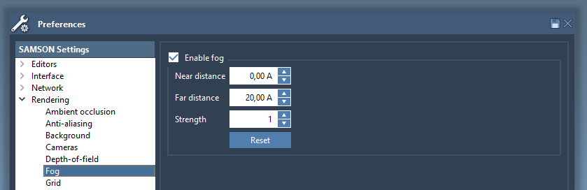
The fog can be switched on/off in one click in the Visualization menu.
Here is 1YRF again with both depth-of-field and fog:
Shadows
Shadows are particularly helpful to improve the perception of relative positions.
Note: In case of an old graphics card you may want to either disable this option, or choose the lower preset.
The shadows settings may be changed in the Rendering / Shadows section of the Preferences panel:
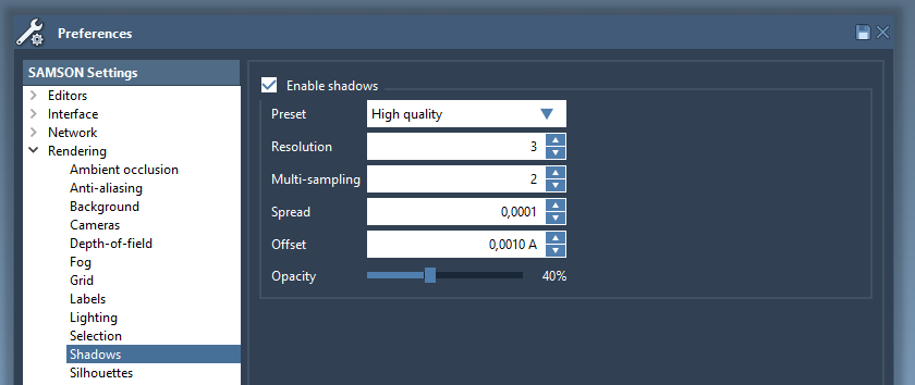
The shadows can be switched on/off in one click in the Visualization menu.
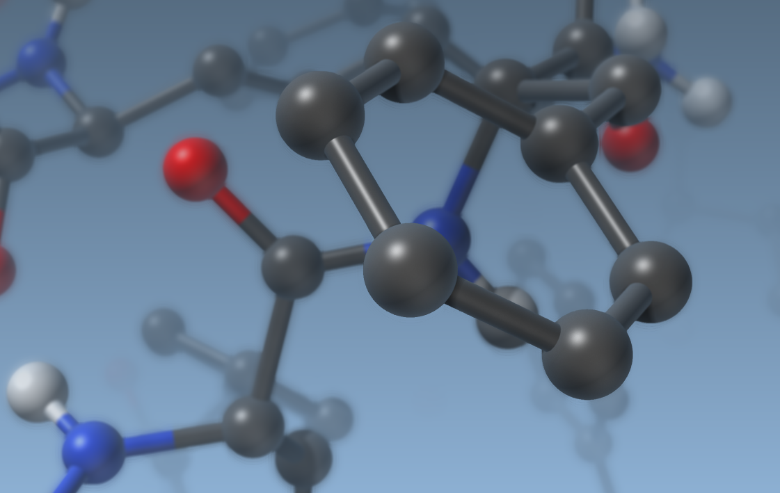
Without shadows, it may be difficult to perceive the relative positions, e.g., of 1YRF to the graphene sheet behind it:
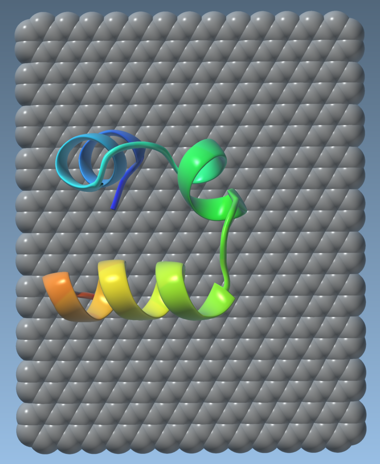
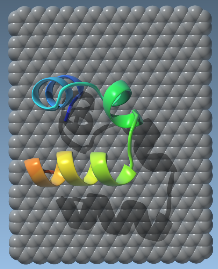
With shadows, however, this becomes much easier:
Silhouettes
Silhouettes make it easier to separate regions with different depths. The silhouettes settings may be changed in the Rendering / Silhouettes section of the Preferences panel.
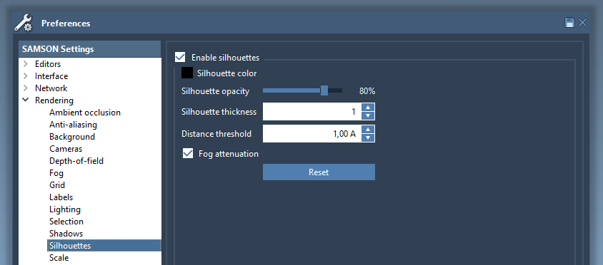
The silhouettes can be switched on/off in one click in the Visualization menu.
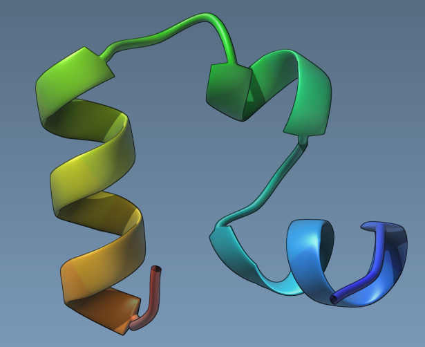
Let's create the Ribbons (secondary structure) visual model for 1YRF molecule and enable silhouettes with the thickness set to 1
Examples
Dengue virus
Let's make the following image of the molecule with PDB code 3J27 (part of the Dengue virus):
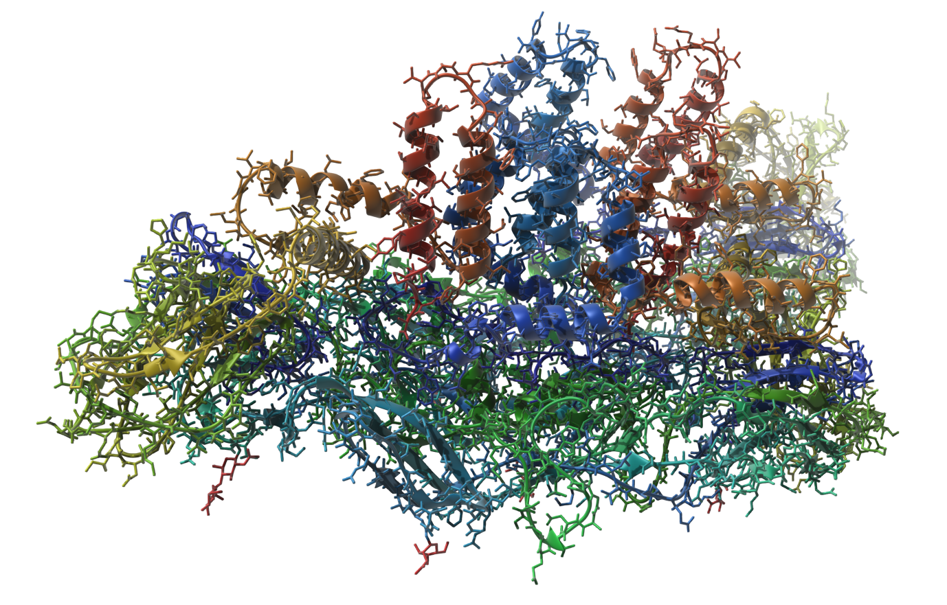
You can reproduce this image via the following steps:
- Add the Ribbons (secondary structure) visual model ( Ctrl/ Cmd⌘ + Shift + V).
- Add the Licorice visual model.
- Hide the structural model of the molecule.
- Position the molecule in the viewport.
- Colorize the Licorice visual model by the residue index (select the Licorice visual model and in the context menu choose Set color > Per attribute > Residue index).
- Ambient occlusion: enable object-space ambient occlusion with the default parameters.
- Anti-aliasing: enable with multisampling factor set to 2, enable FXAA.
- Background: white.
- Fog: enable with the far distance parameter set to 100Å.
- Lightning: default parameters for the first and second lights; set ambient light to 0.
- Shadows: enable with the default parameters.
- Silhouettes: disable.
The nucleosome core particle
Let's make the following image of the molecule with PDB code 1EQZ (the nucleosome core particle):
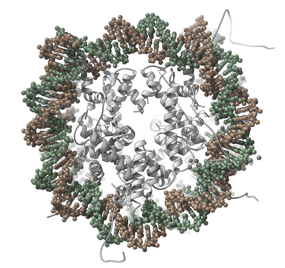
You can reproduce this image via the following steps:
- Position the molecule in the viewport: click on the Back view icon (menu: Visualization > Camera > Back view, Ctrl/ Cmd⌘ + 9).
- In the document view, expand the molecule to see chains. Select chains from A to H and apply the Ribbons (secondary structure) visual model ( Ctrl/ Cmd⌘ + Shift + V), and then hide the selection (right-click, Visibility > Hide selection).
- Select the Ribbons (secondary structure) visual model and colorize it with a constant color (white).
- Open Preferences, modify the structural models representation (Rendering > Structural models): set the atom radius to 1Å.
- Select the chain I and colorize it with a constant color. Colorize the chain J with a constant color.
- Ambient occlusion: disable.
- Anti-aliasing: enable with multisampling factor set to 2, enable FXAA.
- Background: white.
- Fog: enable with the default parameters.
- Lightning: default parameters.
- Shadows: enable with the default parameters.
- Silhouettes: enable and set the silhouette opacity to 60%.
Pilus machine
Let's reproduce an image of the molecule with PDB code 3JC8 (the type IVa pilus machine in a piliated state).
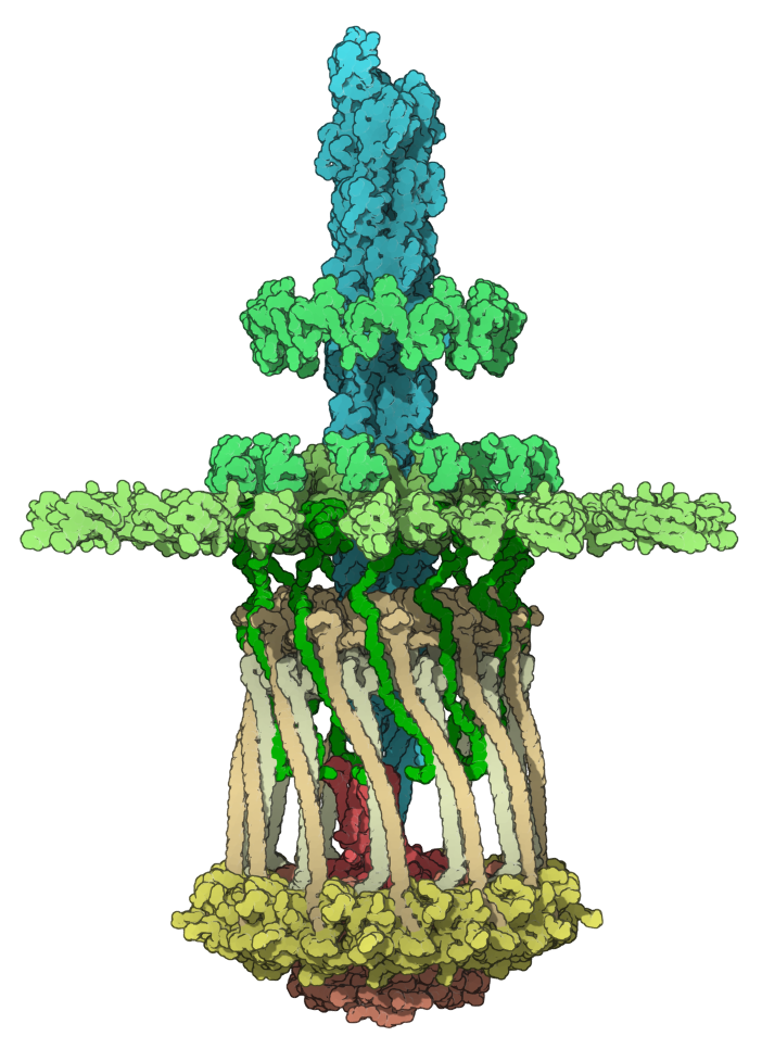
Here we colorized 3JC8 by groups of chains. Please, download 3JC8.sam file in which for simplicity we combined chains in groups.
You can reproduce this image via the following steps:
- Position the molecule in the viewport: click on the Top view icon (menu: Visualization > Camera > Back view, Ctrl/ Cmd⌘ + 8).
- Open Preferences, modify the structural models representation (Rendering > Structural models): set the atom radius to 3Å.
- Colorize each group of chains: double-click on the group and colorize it with a constant color.
- Ambient occlusion: enable object-space ambient occlusion with the default parameters.
- Anti-aliasing: enable with multisampling factor set to 2, enable FXAA.
- Background: white.
- Fog: disable.
- Lightning: the light intensity for first and second lights is set to zero; the ambient light is set to 1 and the Fresnel intensity is set to 0.
- Shadows: enable with the default parameters.
- Silhouettes: enable, set the silhouette opacity to 60%, the silhouette thickness to 1, and the distance threshold to 2Å.
DNA polymerase with DNA
Let's make the following image of the molecule with PDB code 4QWE (DNA polymerase in complex with DNA).
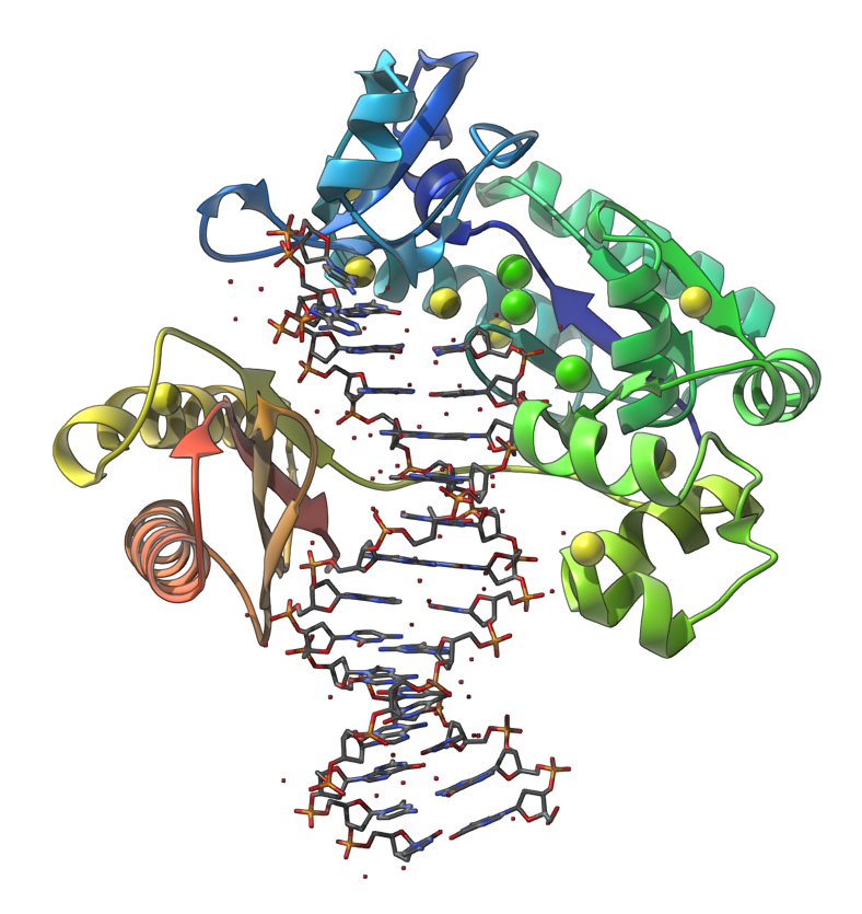
You can reproduce this image via the following steps:
- In the document view, expand the molecule to see chains. Select the chain A and apply the Ribbons (secondary structure) visual model ( Ctrl/ Cmd⌘ + Shift + V), and then hide the selected chain.
- Find all Sulfur and Calcium atoms. Open the Find window (Selection menu > Find or Ctrl/ Cmd⌘ + F). Input
atom.symbol S or atom.symbol Ca(short version:a.s S or a.s Ca) and click Enter. Now you should see 11 nodes selected, press Ctrl/ Cmd⌘ + Shift + V and add Van der Waals visual model. Select in the document view the newly created Van der Waals visual model and in the Inspector (click Ctrl/ Cmd⌘ + I if you do not see the Inspector) set the scale to 0.75. - In the document view, select the chains C and D and apply to them the Licorice visual model.
- Ambient occlusion: disable.
- Anti-aliasing: enable with multisampling factor set to 2, enable FXAA.
- Background: white.
- Fog: enable with the far distance set to 50Å.
- Lightning: default parameters.
- Shadows: enable with the default parameters.
- Silhouettes: enable and set the silhouette opacity to 50%.
The human erythrocyte catalase
Let's make the following image of the molecule with PDB code 1DGF (the human erythrocyte catalase).
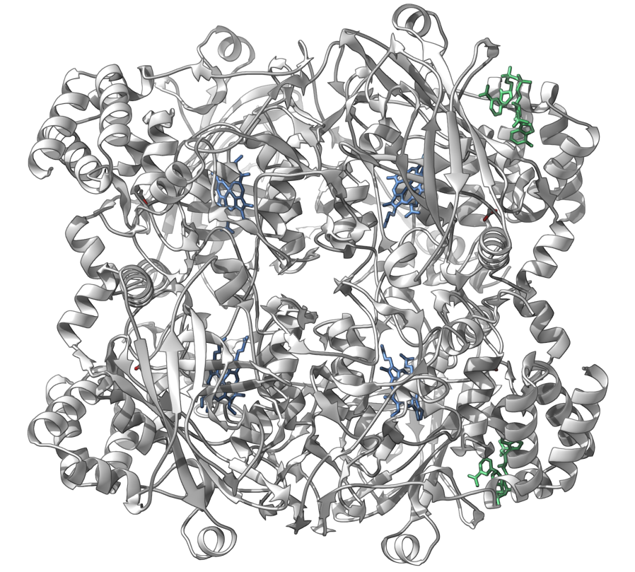
You can reproduce this image via the following steps:
- Add the Ribbons (secondary structure) visual model ( Ctrl/ Cmd⌘ + Shift + V).
- Let's now hide all residues and water atoms, leaving shown only ACT, HEM, and NDP structural groups. Open the Find window (Selection menu > Find or Ctrl/ Cmd⌘ + F). First we will hide all non structural groups: input
n.t structuralGroup(short version:n.t sg) and click Enter, then right-click on any selected node, and choose Invert selection in the context menu, right-click again on any selected node and in the context menu choose Visibility > Hide selection. Let's now hide all water atoms: open the Find window, inputa.waterand click Enter, then right-click on any selected node and in the context menu choose Visibility > Hide selection. - Open Preferences, modify the structural models representation (Rendering > Structural models): set atom and bond radius to 0.3Å.
- In the document view, select the Ribbons (secondary structure) visual model and colorize it with a constant color (white).
- Let's colorize HEM and NDP structural groups. In the document view, enter HEM in the Filter nodes... and click Enter. Colorize it with constant color: right-click on any selected node and in the context menu choose Set color > Constant. Do the same for the NDP structural groups.
- Ambient occlusion: disable.
- Anti-aliasing: enable with multisampling factor set to 2, enable FXAA.
- Background: white.
- Fog: enable with the far distance set to 50Å.
- Lightning: default parameters.
- Shadows: enable with the default parameters.
- Silhouettes: enable and set the silhouette opacity to 50%.
- Position the molecule in the viewport.
See also: Color schemes See also: Visual models See also: Visual presets See also: Presenting and animating